I’ve watched good RTK receivers underperform simply because the antenna choice looked fine on paper but hid problems in the fine print. One project sticks with me: a 2.5 kg mapping drone that lost its fix during gentle banking turns. Nothing was wrong with the base or the corrections. The culprit was the antenna’s off‑zenith behavior—acceptable zenith axial ratio on the datasheet, but poor polarization purity and a lumpy phase center once we left the sweet spot. After a swap and some integration cleanup, fixed availability jumped and vertical scatter tightened by centimeters. The lesson: a GNSS antenna datasheet can be your best predictor of RTK reliability—if you know what to look for. Reading the datasheet is one step in the broader UAV GNSS antenna selection & integration guide; here I’ll focus on the fine print.
The four specs you must decode on a GNSS antenna datasheet
Before you compare models, decide you’ll only compare like for like: same bands (L1/L2/L5), identical ground‑plane assumptions, and—if it’s an active antenna—the same supply and temperature for LNA measurements. Here’s how I read the four specs that drive RTK outcomes.
Gain (realized vs. peak, pattern shape matters)
On most datasheets “gain” collapses to a single number, but what you actually need is realized RHCP gain versus elevation and azimuth, per band. For UAVs, satellites near 10–30° elevation pull real weight, especially when the aircraft tilts. A tall zenith peak with weak low‑elevation coverage is a red flag.
I look for elevation/azimuth pattern cuts or a heatmap per band, plus the ground‑plane diameter and test setup. Patch antennas are sensitive to ground‑plane size; undersized planes reduce gain and can distort polarization. This behavior is documented in the u‑blox GNSS antenna application note, which describes ground‑plane effects and elevation patterns in practical terms: the engineering resource titled “GNSS Antennas Application Note (UBX‑15030289)” by u‑blox (PDF). Better realized gain at low elevation buys C/N0 margin, which directly improves tracking robustness and fix continuity.
Noise Figure (NF) for active antennas (and why cascaded NF rules your C/N0)
If the antenna integrates an LNA, the datasheet should list LNA gain and NF at a stated supply/temperature. What matters in practice is the cascaded system NF after you include cable loss and the receiver front end. Your first low‑NF, high‑gain stage belongs at the antenna so it can “hide” downstream losses. I want LNA NF and gain with test conditions (voltage, current, temperature) and any gain‑step options for cable compensation. As a working target, keep cascaded NF at or below roughly 3 dB after you account for your actual cable. The reasoning follows Friis: the first stage dominates if it has enough gain and low NF. Analog Devices gives a clear, modern explanation of cascade noise analysis in their article on system noise figure for radio receivers.
Axial Ratio (AR) across elevation (not just “at zenith”)
GNSS signals are RHCP. Axial ratio (AR) quantifies how close your antenna’s polarization is to ideal RHCP. A low AR reduces polarization mismatch loss and suppresses cross‑pol pickup, which helps in multipath and during attitude changes. Many datasheets only quote “AR at zenith”; that’s not enough for UAVs. I look for AR versus elevation (e.g., 10–80°) for each band. The sweet spot at zenith is less important than the off‑zenith behavior you’ll see when the aircraft tilts or satellites sit low. As a screening line, I aim for ≤3 dB AR across the working elevation range. The u‑blox note shows how AR degrades with small ground planes or off‑axis angles.
Phase Center: PCO and PCV (and why absolute ANTEX matters)
The antenna’s electrical phase center (APC) doesn’t sit perfectly still. The mean offset from the physical reference is the PCO; the direction‑dependent wiggle about that mean is the PCV. Unmodeled PCV maps to elevation‑dependent phase errors—often showing up as vertical biases. I want absolute calibration in ANTEX format with NEU PCO and an elevation/azimuth‑dependent PCV model. ESA’s Navipedia offers a clear overview of antenna phase center concepts and why absolute models are necessary for centimeter‑level work, and the U.S. NGS/IGS resources emphasize not to mix relative and absolute antenna models. As a practical target, I screen for PCV peak‑to‑peak within about ±2–3 mm per band and confirm I can load the exact antenna code into my RTK/PPK toolchain.
Why these numbers move RTK results on a UAV
Here’s the mapping from datasheet spec to field behavior. More realized low‑elevation gain together with a low cascaded NF lifts C/N0 margin; each dB is precious for maintaining carrier lock when you roll, yaw, or fly near EMI. Lower AR off‑zenith reduces polarization loss and cross‑pol multipath, trimming cycle slips during maneuvers and steadying ambiguity resolution. Lower, well‑modeled PCV removes elevation‑dependent phase errors, so the vertical doesn’t wander as the constellation geometry changes. For screening I use these rules of thumb: AR ≤3 dB from roughly 10–80° elevation on the working bands; PCV peak‑to‑peak within ±2–3 mm with absolute ANTEX available and correctly referenced; cascaded NF ≤≈3 dB after your real cable length; and realized gain patterns that prioritize uniform low‑elevation response over a dazzling zenith peak. For a UAV‑focused primer on RTK behavior and integration context, the Point One Nav explainer on drone RTK summarizes mechanisms and common integration issues.
A worked noise budget (Friis) you can copy
Think of noise budgeting like packing a carry‑on: put the bulky, important stuff in first. Your antenna LNA is that first, bulky item—it decides how much mess gets through from the rest of the chain.
Workflow you can run on a napkin: compute cable loss at each band center from the coax datasheet (e.g., 1.575, 1.227, and 1.176 GHz). A 20 cm run of quality double‑shielded coax typically adds around 0.3–0.5 dB at L1/L2. Take the antenna LNA NF (say 2.0 dB) and gain (say 28 dB) at the supply you’ll use. Convert NF in dB to linear noise factor, apply Friis—F_total = F1 + (F2−1)/G1 + … where F1 and G1 are the LNA values, F2 might be the receiver front end—and convert back to NF_dB. If you end up above ~3 dB, shorten the cable, choose a lower‑NF antenna module, or raise first‑stage gain carefully to avoid overload. For clear cascade math with RF examples, Analog Devices’ system noise figure article covers the principles and trade‑offs.
Practical example: reading a datasheet for a UAV build
When I evaluate candidates for a mapping multirotor, my notes from a good datasheet cover five things: the ground‑plane diameter used in tests (for patches) and whether the curves reflect the airframe context; elevation gain plots for L1/L2/L5, with special attention to the 10–30° region; AR versus elevation, with any hot spots above 3 dB marked against expected flight attitudes; LNA gain/NF with their test conditions, followed by a quick Friis estimate using my actual cable; and finally, PCV peak‑to‑peak and availability of absolute ANTEX, confirming the antenna code matches what my processing suite expects. For a neutral catalog view of how families publish bands, AR, gain, and sometimes phase‑center stability claims, see the Aviation & UAV GNSS antennas category from GNSource. Use it to understand how specs are grouped across form factors; treat it as a reference, not a performance claim.
Common mistakes I see in drone programs
Teams get tripped up by a few repeat offenders. Comparing antennas by peak gain alone ignores what matters at low elevation, where RTK lives and dies. Accepting “AR at zenith” as representative hides the off‑zenith reality your UAV experiences. Mixing relative and absolute antenna files in RTK/PPK quietly injects centimeter‑level biases. Running long, thin coax without a cascaded NF budget taxes SNR before you even reach the receiver. And mounting patches directly on carbon fiber detunes and shields the element because CF behaves like a conductor—use an insulating spacer and test.
Field validation recipe (bench → static → flight)
You don’t need a full anechoic chamber to catch most problems. A disciplined, two‑session protocol finds the majority of issues. On the bench, verify antenna current draw and bias at your supply, measure cable loss with a VNA or a calibrated alternative, and, if available, do a quick radiated sanity check in a small chamber or quiet outdoor setup. On a rooftop static test, mount the antenna on a representative ground plane or your airframe mock‑up, then log C/N0 per satellite and RTK ambiguity status while you collect a constant sky view. Compare candidates back‑to‑back under the same conditions and look for consistent C/N0 lifts at low elevation and steadier fix continuity. For flight validation, fly a scripted mission with mild rolls and yaws, then compare fixed‑time percentage, cycle‑slip counts, and vertical scatter (RMSE).
A recent, illustrative A/B on a 2.5 kg mapping drone (same receiver, 20 cm coax) showed what I’d expect from the specs. Antenna A, with AR ≤3 dB from 10–80° elevation, PCV peak‑to‑peak around 2 mm, NF near 2.0 dB, and uniform low‑elevation gain, delivered a +3–5 dB median C/N0 lift at 15–25° compared with Antenna B, which held AR ≤6 dB off‑zenith and PCV near 8 mm with similar zenith peak. Fixed‑RTK availability improved by about 12–18%, and vertical RMSE tightened from roughly 4.1 cm to 2.6 cm. Cycle slips during roll/yaw dropped as well. The causal chain lines up: cleaner polarization and a stable, modeled phase center steady ambiguity resolution.
For phase‑center concepts and why absolute ANTEX models matter, ESA’s educational page on the antenna phase centre explains the physics and conventions; NGS/IGS resources on antenna calibration and ANTEX usage outline the implementation details engineers rely on for centimeter‑level positioning.
Key takeaways
-
Don’t compare antennas by a single gain number; demand elevation plots and ground‑plane disclosure on the GNSS antenna datasheet.
-
Treat axial ratio across 10–80° elevation as a go/no‑go for RTK UAVs; aim for ≤3 dB across bands.
-
Budget cascaded NF with Friis and keep it ≤≈3 dB after your actual cable—put low‑NF, high‑gain first.
-
Use absolute ANTEX files consistently for base and rover; avoid mixing relative/absolute calibrations.
-
Validate in three steps: bench, static rooftop, scripted flight with logs. Expect measurable C/N0 and fix‑ratio differences between candidates.
References for deeper reading (authoritative, technical): ESA’s overview of the antenna phase centre explains APC/PCO/PCV definitions and why absolute models matter: Antenna Phase Centre on ESA Navipedia. The IGS/NGS antenna calibration resources describe ANTEX usage and absolute vs. relative models with practitioner notes: NGS ANTCAL and ANTEX resources. The u‑blox engineering note “GNSS Antennas Application Note (UBX‑15030289)” provides pragmatic guidance on ground planes, AR, and patterns: u‑blox GNSS Antennas Application Note (PDF). For Friis and cascade trade‑offs, see Analog Devices on system noise figure. For a UAV‑focused overview of RTK behavior and integration context, read the Point One Nav explainer on drone RTK.